Palletizing a mixed order is an NP-hard problem. A hundred boxes of different sizes can be arranged in more ways than a computer can check. So people use heuristics, rules that find a good solution quickly without guaranteeing the best one.
Research on pallet building usually solves each order on its own, without looking at the truck or the route. Work on vehicle routing with loading constraints does consider the whole truck and the unloading order, but it loads loose boxes or single-customer pallets. Few studies build the pallets and place them in the truck at the same time1.
Distribution needs both at once. What leaves on a route is a truck carrying the orders of several customers, split over pallets that mix customers and are loaded in reverse stop order. At each stop, the driver's helper pulls one customer's boxes without taking apart the next customer's.
We needed a system that could build anything from one pallet to a full truck. At its core is a solver, the program that decides which box goes where. On a test fleet of 80 trucks of about 500 boxes each, the solver planned each truck in a median of 170 milliseconds. On 50 test orders whose best solution we knew, it used one extra pallet on 45.
What palletizing a mixed order means
Each order line is a SKU, a product with its own box size. Several SKUs can share a box size. A single-SKU pallet is built by repeating the same layer. When an order mixes products, each layer combines boxes of different sizes, and someone has to decide where each one goes. Figure 1 shows three pallets built by our system, with one, three and nine SKUs.
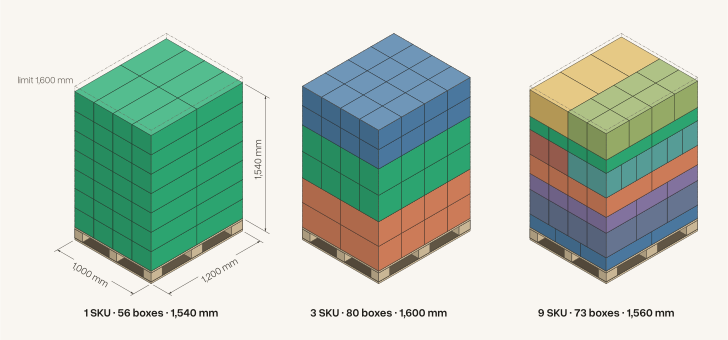
Figure 1. Each colour is a SKU and the dashed line marks the 1,600 mm limit. For each case we picked, from about 300 generated orders, one with box sizes that divide the pallet base. They are favourable orders, and Figure 12 shows a typical one.
Formally, an order is a set of boxes, each with dimensions and mass . The task is to split it into pallets and give each box a position that keeps it inside its pallet's volume without overlapping other boxes, using the smallest possible . We use pallets of mm and mm.
If every box had the full pallet base, only their heights would matter. The boxes would have to be split over the fewest pallets with on each, which is one-dimensional bin packing, strongly NP-hard. The general case contains that special case, so it is NP-hard too.
The formal model leaves out four conditions that a pallet to be picked from has to meet.
- Pick groups. Boxes of the same SKU for the same customer stay together, in a block that can be pulled at the stop.
- Physics. Every box needs support, heavy boxes go below and the pallet respects its maximum height and weight. Boxes can turn 90° about their vertical axis, but they are never tipped over.
- Operating rules. Every company has its own, such as separate temperatures, route order or customers with dedicated pallets. The solver takes them as configuration.
- Time. The plan is computed with the route closed and the trucks waiting.
The support of a box is the share of its base that rests on top of other boxes,
where is the area where the bases of and overlap seen from above, and mm is the contact tolerance. A box on the pallet has . We call a box well supported when , the usual threshold in routing with loading constraints2, and count it as floating when , a category of our own. Figure 2 shows the three levels.
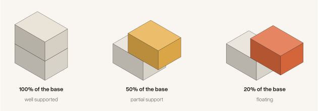
Figure 2. A box on top of another with 100%, 50% and 20% of its base supported, in the same colours as Figure 12.
The unit of work is a truck
A truck in the test fleet carries about 10 pallets of 1,000 × 1,200 mm and about 500 boxes for ten customers, one stop per customer (Figure 3). The solver builds all of its pallets at once, and the system then orders them by route.
If is the stop of box , a pallet's first delivery is . Pallets are loaded from the highest to the lowest , alternating between the two columns. The pallet at the back, against the cab, is therefore the one that starts unloading last.
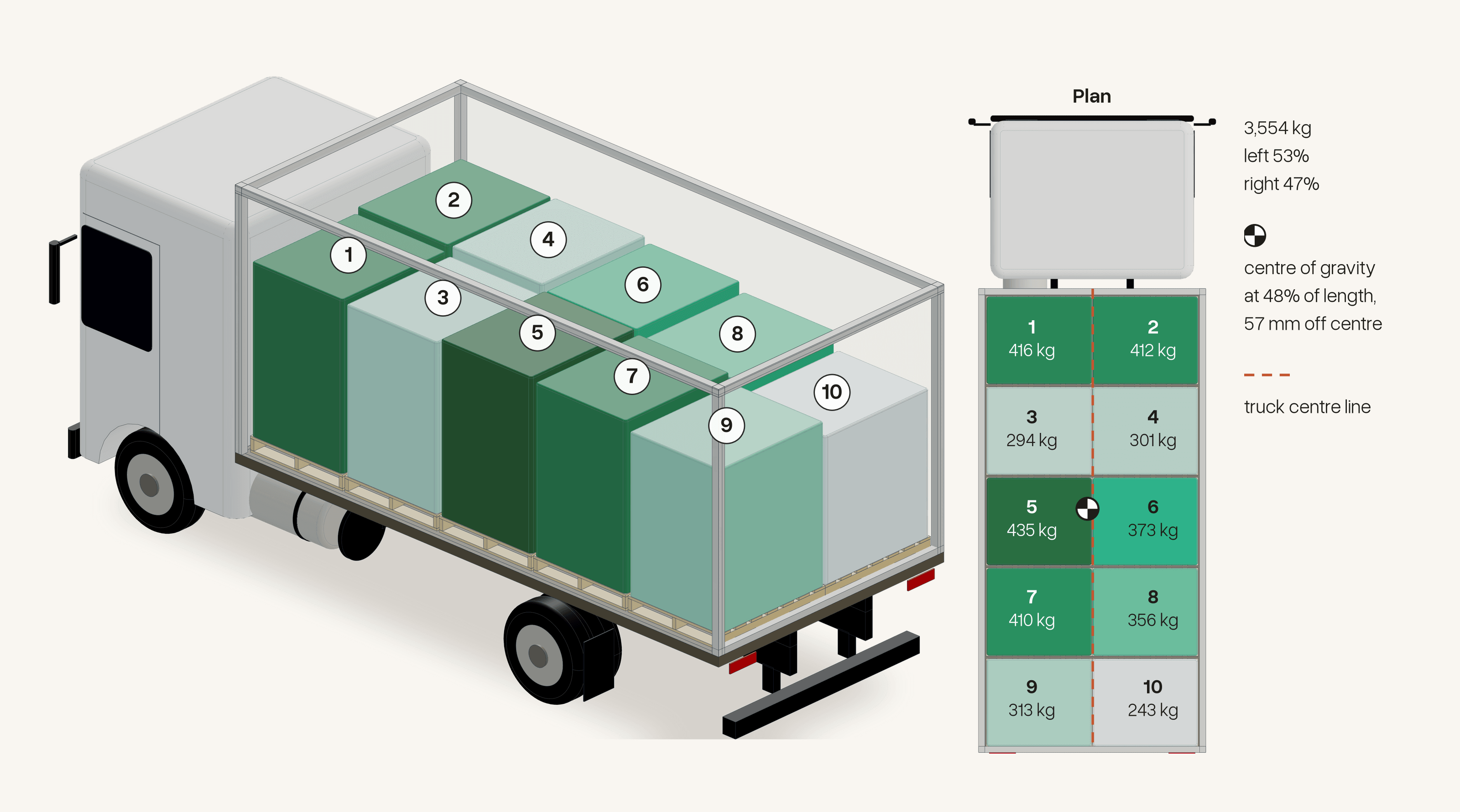
Figure 3. A truck from the test fleet, modelled in CAD with its 10 pallets at the position and height the solver returns. Each pallet's number is its load order, from 1, against the cab, to 10, by the doors. Colour shows weight, from 243 to 435 kg, and the plan shows each pallet's weight and the load's centre of gravity. We chose the truck whose left/right weight difference is closest to the fleet median (Figure 9).
How we build the pallets
The operation's rules define which boxes may share a pallet. Within those limits, the solver decides how many pallets to build and what goes on each.
Trying box by box would be too slow. We checked with an engine that places each box in the free corners of the surface built so far and applies published support rules. It left no box floating, but it built 2,969 mm columns on pallets with a 1,600 mm limit and took more than ten minutes on a test set, so we dropped it.
The solver works with larger pieces. It groups the identical boxes of each pick group into blocks, builds layers from those blocks and stacks the layers into pallets (Figure 4). Building with blocks and layers is one of the oldest ideas in the loading literature3. With blocks, each pick group also stays in one piece.
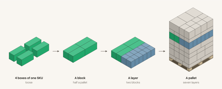
Figure 4. From box to pallet, on the nine-SKU pallet of Figure 1. The four green boxes form a half-pallet block. That block and one of twelve blue boxes form a layer, and seven layers form the pallet.
Each layer comes from a beam search. At every step, the solver extends several partial layers with one more block, compares the results and keeps only the best (Figure 5). That way it does not commit to an early choice that later leaves gaps.
If is the set of partial layers it keeps at step , the next step is
where is the set of blocks that fit in the free space of layer , is the layer with the block added and keeps the best by a coverage and contact score. With it would be a greedy algorithm, and with unlimited , an exhaustive search.
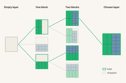
Figure 5. Simplified schematic of a beam search that keeps two partial layers per step, using the blocks of the layer in Figure 4. At the first step there are three options for two places and one is left out. At the second, each kept option is extended in two ways, and the two that leave gaps are dropped.
When layers are stacked, a layer can repeat the seams of the one below. If that happens over several layers, the pallet splits into columns and its stability depends on the film alone. So the solver rebuilds mixed layers to cross the seams of the layer below, the way bricks are laid in a wall4 (Figure 6). Full single-SKU layers are not rebuilt, and those stretches stay in columns.
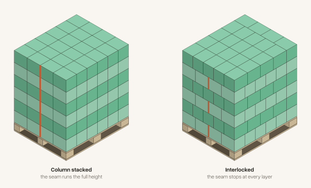
Figure 6. Schematic of 144 identical boxes stacked two ways. Column stacked, every layer repeats the same pattern and the marked seam runs the full 1,200 mm of cargo. Interlocked, layers alternate between two patterns and the same seam stops at every layer.
Finally, the solver settles every box where gravity leaves it and measures again how much of its base is supported. When an order cannot satisfy a rule and a physical limit at the same time, it returns the best plan it finds and flags the pallet that exceeds the limit.
How we used AI to build it
We built the solver over seven months together with coding agents. We defined the problem, the rules of each operation and what counts as a good pallet. The agents wrote the solver's code, the experiments and the tools to measure them.
What changed most was how fast we could test ideas. Every idea goes through the same loop (Figure 7). An agent implements it, runs the solver on batteries of test orders and measures every pallet box by box. We review the results and decide whether the idea stays. Several ideas can go through the loop in parallel, and a variant of the build can be designed, measured and dropped within a single day.
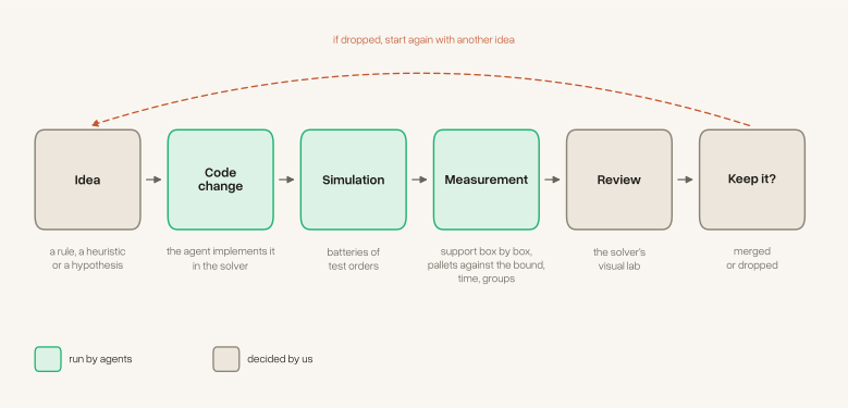
Figure 7. The loop we use to test each idea in the solver. In green, the steps agents run, and in beige, the ones we decide.
That pace let us test theories we would not have had time to test by hand. More than a dozen ideas were dropped, each with its measurement written up. Several improved one measure and worsened another, such as the pallet count or the solve time. The agents also built physical simulations of the pallet and the interfaces we use to review the solver, such as a visual lab that replays step by step how each pallet was built. With them, each change is reviewed by looking at the pallets it produced as well as at their averages.
This way of working has a clear limit. When the optimal solution is unknown, agents can only improve the metrics we give them, and a metric can look good on a pallet that does not work. The free-corner engine left no box floating and still built columns over the height limit. Knowing whether a pallet is stable and can be picked from still depends on looking at it, and there even the most capable models we used are not reliable. That is why visual review and the decision on each change stay with people.
In total we used about 50 billion tokens, worth about US$20,000 at list prices.
Results on the test fleet
The test fleet has 80 trucks with orders from BED-BPP, a public set of real grocery orders5. Each truck carries ten customers, and the fleet adds up to 40,776 boxes. The solver planned all of it in 13.7 seconds, on one core of an Apple M4 laptop. It used 798 pallets, with no box left out and no pallet over the limit. 81.7% of boxes ended up well supported and 1.1% floating.
Each truck took between 100 and 290 milliseconds, with a median of 170 (Figure 8). With 16 trucks in parallel, and if time scaled with no losses, the fleet would take under a second. These times exclude database reads and writes.
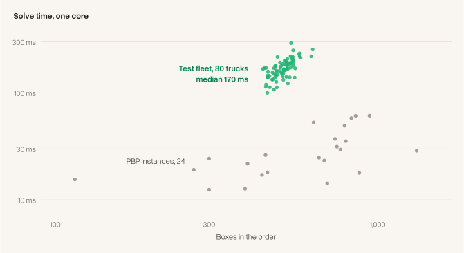
Figure 8. Solve time against boxes per order, on a log scale. In green, the 80 trucks of the test fleet (median of 3 runs). In grey, the 24 instances of the public PBP benchmark, which we compare below (median of 5).
Two studies that model practical constraints report times of another order. One, with instances generated from a logistics provider's data, reports about a minute of computation per pallet, within its industrial partner's two-minute standard per plan. Another builds layers with heuristics and then assigns them to pallets with an integer program. On its three largest orders, of 332 to 669 boxes, it hit the 120-minute limit in every run. At a minute per pallet, run in series, the 798 pallets of our fleet would take more than 13 hours.
The load order follows the route and ignores weight. If and are the masses to the left and right of the truck's centre line, the left/right difference is . The fleet median of is 5%. On 10% of trucks it exceeds 13%, and on the worst it reaches 24%. The centre of gravity along the cargo, , always fell between 40% and 56% of the length, measured from the cab (Figure 9).
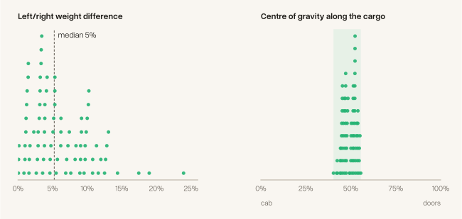
Figure 9. On the left, the left/right weight difference on each of the 80 trucks of the fleet. On the right, the position of the centre of gravity , from the cab to the doors.
To judge the 798 pallets we compare them with a lower bound. A truck's bound is
the volume of its load divided by the usable volume of a pallet, rounded up. No plan can use fewer pallets. Summed over the 80 trucks it comes to 565. The gap to 798 comes partly from the solver and partly from the bound, which ignores the shape of the boxes, and we cannot tell how much each contributes.
How far from the optimum
The lower bound does not say how much of the gap is the solver's. Measuring that takes an order with a known answer. We built 50 orders by cutting full pallets into layers of identical boxes, with 1 to 16 pallets per order. The optimum is the number of pallets cut, and if the solver uses , the relative gap is .
The solver hit the optimum on 2 orders, used one pallet more on 45 and two more on 3. It left no box out, and 99% of boxes ended up well supported. Its pallets were 90% to 95% full. What does not fit ends up on an extra pallet that is 7% to 73% full (Figure 10).
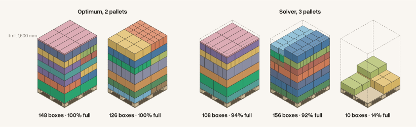
Figure 10. A test order cut from two full pallets, on the left as it was cut and on the right as the solver built it. Each colour is a SKU. The solver left its first two pallets 94% and 92% full, and the 10 boxes that did not fit went to a third pallet.
The table groups the 50 orders by size, with ten orders per row.
| Pallets in the optimum () | Boxes per order | Solver pallets (, mean) | Extra pallets () | Relative gap |
|---|---|---|---|---|
| 1 | 119 | 1.9 | 0.9 | 90% |
| 2 | 255 | 2.9 | 0.9 | 45% |
| 4 | 462 | 5.0 | 1.0 | 25% |
| 8 | 968 | 9.0 | 1.0 | 13% |
| 16 | 1,895 | 17.3 | 1.3 | 8% |
Since the difference stays close to one pallet, the relative gap falls roughly as , from 90% on 1-pallet orders to 8% on 16-pallet orders.
A public benchmark
As an external reference, we ran the solver, unchanged, on the 24 pallet building problem (PBP) instances of Calzavara et al. (Annals of Operations Research, 2025). They come from a real case at a company that builds robotized pallet-building systems, and they also require items of the same type to stay grouped. Our solver used 9.79 pallets on average, in 30 milliseconds per instance. The paper's fastest algorithm uses 11.29 pallets in the same time, and the one that uses the fewest, 9.97 with 15 minutes of search (Figure 11).
The comparison is approximate, and the rule differences cut both ways. Those algorithms must build full horizontal layers and satisfy visibility rules that ours does not impose, and ours requires a minimum support for every box. They also ran on other hardware6.
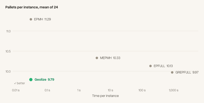
Figure 11. Average pallets against time per instance, on a log scale, on the 24 Calzavara et al. instances. EPMH, MEPMH, EPFULL and GREPFULL are the paper's variants, from fastest to most exhaustive. The lower bound averages 7.6 pallets. Rules and hardware differ (see text).
What box variety costs
In the single-SKU pallet of Figure 1, each box rests fully on the one below. With many box sizes, layers can end up at uneven heights and with gaps (Figure 12). A truck in the fleet mixes a median of 132 box sizes.
With such heterogeneous cargo, many methods stop building layers and place boxes one at a time7. We keep the layers, so we measured what that costs us with real grocery boxes and with pick groups kept together.
To isolate the effect, we built 1,320 synthetic orders with real boxes from BED-BPP. The load of each order equals 80% of 1, 2 or 4 pallets. Within each size, only the number of box sizes changes, from 1 to 48, with 40 orders per combination.
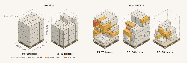
Figure 12. Two orders with the same load, about two pallets. Colour shows how much of each box's base is supported, grey for 75% or more, amber for 30% to 75% and red below 30%. From each group of 40 we chose the most typical order. With one size, 166 boxes fit on 2 pallets and all are well supported. With 24 sizes, 162 boxes take 3 pallets and 77% are well supported.
Support falls as variety grows (Figure 13). In 2-pallet orders, well-supported boxes drop from 100% with one size to 77% with 24 (95% interval, 75–78%)8. With 48 sizes they reach 71%. Floating boxes go from 0% with one size to 3.9% with 24. Small orders lose more, and with 48 sizes a 1-pallet order leaves only 58% of its boxes well supported.
Variety also costs pallets. With one size, 2-pallet orders used 2.1 pallets on average, and with 24 sizes they used 3.0, one more than the lower bound on every order. Density measures how much of the pallets' volume, up to their real height, the boxes fill. If is the volume of the boxes and the height of pallet , it is . It fell from 88% with one size to 70% with 24.
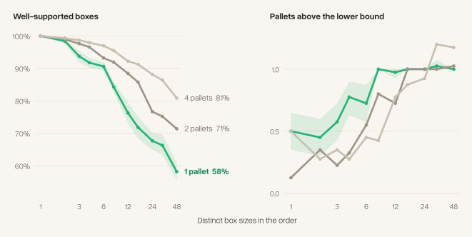
Figure 13. Each point averages 40 orders with the same load, and the green band is the 95% confidence interval. On the left, the share of well-supported boxes. On the right, the pallets each order uses above the lower bound. 1-pallet orders, in green, lose the most.
Some sizes appear once and others dozens of times, so to compare the fleet with the experiment we measure variety with the entropy of the mix. If is the share of boxes of size , the entropy and the effective number of sizes are
is the number of equally common sizes that would give the same entropy. In the synthetic orders quantities are nearly even, so 24 sizes are worth about 21.
The 132 sizes of a typical fleet truck are worth 89, more than any order in the experiment. Even so, the fleet left 81.7% of its boxes well supported, almost the same as the four-pallet synthetic orders with 48 sizes, which reached 81%. Large orders lose less support, and a truck in the fleet carries about 10 pallets.
We think the cause is the one Figure 12 suggests. A size that appears only a few times cannot fill a layer, its boxes end up in mixed blocks, and those blocks leave uneven heights. We did not test this explanation separately, and we do not know whether another method would lose support at the same rate.
The rules of each operation
An operation's rules cost pallets, and they cost more as the truck mixes more box sizes. We measured it on 120 synthetic six-customer trucks with 6 to 48 box sizes, and solved each one under different rule combinations.
The measure is , the pallets used per pallet of load volume. If every pallet reached the maximum height, would be the inverse of . With only the pick-group rule, rises from 1.36 with 6 sizes to 1.79 with 48. With all the operation's rules, among them separate temperatures and route order, it rises from 1.69 to 2.47 (Figure 14).
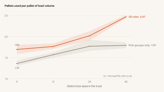
Figure 14. Pallets used per pallet of load volume, on synthetic six-customer trucks, 30 per point. The band is the 95% confidence interval.
A rule can collide with a physical limit. With a rule that keeps each customer's boxes together, 88 of 320 pallets ended up over the maximum height, because some customers did not fit on one pallet. The solver kept the rule, flagged those pallets and leaves it to the operation to decide which one gives way.
Building the pallet in the warehouse
Picking is building the pallet in the warehouse. A picker walks the locations with an empty pallet, takes out the boxes of each order and stacks them layer by layer. The solver's plan says where each box goes and in which layer. Building from the bottom up, each box lands on one that is already in place.
The simulator builds a pallet this way, one the solver planned for a test order with three customers and seven SKUs. Each customer's boxes sit in consecutive layers, and the customer delivered last goes at the bottom. The picker takes the boxes of one SKU, places them and moves on to the next, and the pick list shows those steps customer by customer. You can play it, step through it box by box, jump to a SKU or turn the pallet.
Loading the simulator…
Empty pallet
Pick list
Drag the pallet to turn it. Tap a SKU to jump to that step.
Simulator. A pallet from the solver, 69 boxes in seven full layers, built from the deck in an order a picker could stack it in. Each customer has a colour family and each shade is a SKU. While a SKU is being picked, the rest of the pallet fades back, and the pick list marks one step per SKU and layer.
A pallet can be picked from if each pick group comes out in one piece. We measure it with the same connection rule the solver applies, so this is a consistency check. Two boxes of a group are joined if they touch, or if a short gap with no box of another group separates them9.
In the fleet, more than half of the groups are a single box. Of the 10,148 groups with two or more boxes on a pallet, 98.0% formed one block. Of all groups, 1.1% were spread over several pallets. Large groups split more often. In the synthetic trucks, where groups have dozens of boxes, 79% to 84% of them formed one block. Figure 15 shows a pallet with two split groups.
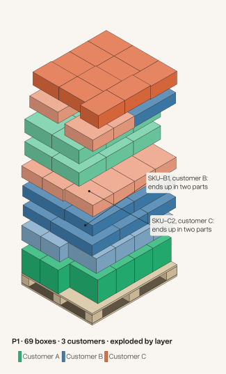
Figure 15. A pallet from a test order with three customers, separated by layer to show its interior. Each customer has a colour family and each shade is a SKU. Two of its six pick groups ended up in two parts, as the callouts show. The order's second pallet has all six groups in one block.
What happens at each stop
On the route, the truck's helper takes out each customer's boxes at their stop. The pallets are loaded in reverse route order, so those for the first stops sit by the doors (Figure 3). The plan also says which pallet and which layer each box goes on, so at every stop the helper knows in advance which pallets to open.
Each SKU comes out in one piece. A customer in the fleet receives a median of 52 boxes of 26 SKUs, and the helper takes them out in a median of 27 blocks, almost one per SKU. That is the result of keeping pick groups together while building.
Because orders are small, the solver mixes customers to fill layers, and a customer's boxes end up on a median of 7 pallets. Mixing is a cost decision, since rules that group boxes by route or by customer cost pallets. With all the operation's rules, rises from 1.36 to 1.69 with 6 box sizes (Figure 14). Each operation chooses what suits it, and the solver builds with either configuration.
What these results do not show
- Physics is modelled by support area, not measured. We do not check each box's equilibrium or the effect of stretch film.
- Full single-SKU layers stack in columns. In those stretches a straight seam can run the whole height of the pallet, and stability depends on the film.
- We do not compute axle loads. We report the centre of gravity at departure, but the legal test depends on each truck and the distribution changes at every stop. In one routing study, ignoring axles left more than 25% of the loaded arcs over some limit10.
- We do not re-measure support after each stop. Pulling one customer's groups can leave the remaining boxes without support.
- Stop order within a pallet is not guaranteed. Pallets are loaded by route, but within a pallet the first customer does not always end up on top.
- We did not measure time on the route. Mixing customers fills layers with fewer pallets, but the helper opens more pallets at each stop. We did not measure how much time that adds.
What comes next
Building pallets has no fixed solution. The best pallet depends on the operation that uses it, on its boxes, its rules and what happens to the pallet after it is built. That is why we work on the solver every day, and every change is measured against test orders before it goes in. Sometimes that means adjusting it to an operation's requirements. Most of the time we aim at the same thing, pallets that are built fast and that work for picking.
Our focus is pallets built to be picked and sent out on a route the same day. There, what matters is speed, each pick group in one block and every box well supported. A pallet that will sit stacked in a warehouse for months is a different problem, and the literature covers conditions that weigh less in our case11.
- Strength of each box. Models with load-bearing strength cap the weight each box can carry before it crushes12. The strength of a corrugated box depends on the board, on humidity and on how long it stays under load13, so it is decisive for stored pallets. On a pallet that travels for hours it matters less, and the solver approximates it by putting heavy boxes at the bottom. We are studying it for operations that have that data per SKU.
- Stability in motion. Measuring how a load behaves through braking and turns requires simulating the trip14. We measure the static support of each box, and holding the load on the road is left to the stretch film.
- Exact models. Integer programming models that include support and load bearing only solve problems of moderate size15. With the route closed and the truck waiting, we prefer a heuristic that answers in milliseconds, and we measure how far it lands from the bound.
What occupies us most today is small orders with many box sizes, the case the literature recognizes as the hardest to build in layers. For it we are working on compact blocks with a few boxes of each size, to fill the gaps between layers. We also want the route to count while building, to bring each customer's boxes onto fewer pallets without losing full layers. If your operation builds mixed pallets that are picked later, talk to us.
Notes
- On pallet building, see Gzara, Elhedhli and Yildiz (2020) and Calzavara et al. (2025). On routing with loading constraints, Iori and Martello (2010) and the review by Pollaris et al. (2015). Alonso et al. (2016) build pallets and load them into trucks at the same time, for transport between depots, with no multiple stops and no pick groups. We know of no work that builds pallets shared by several customers on one route, although our search was not exhaustive. The problem is NP-hard because it generalizes bin packing (Dell'Amico and Magnani, 2021).
- Miao et al. (2012) describe 75% support as the standard requirement in three-dimensional routing with loading, and Gzara, Elhedhli and Yildiz (2020) use 70%. Support under each box does not guarantee that the whole stack is stable, because that depends on the centre of gravity of the whole (Krebs, Ehmke and Koch, 2021).
- Layers and walls go back to George and Robinson (1980). The beam search for building layers follows Araya and Riff (2014), Araya, Moyano and Sánchez (2020) and Fanslau and Bortfeldt (2010).
- Carpenter and Dowsland (1985) formalized the criterion of interlocking layers so that seams do not repeat.
- Kagerer et al., BED-BPP, a robotic packing benchmark with 10,003 real grocery orders. We use its 1,730 distinct box sizes, with their weights and how often each appears.
- The published algorithms ran on a virtual machine with a 2.0 GHz Xeon, and ours on one Apple M4 core. Besides horizontal layers, those instances require a residual layer on top, minimum fill factors and that every item be visible from one side. The lower bound we compute (7.62 pallets on average) matches the paper's (7.63).
- Zhao et al. (2016) note that with strongly heterogeneous cargo, methods usually place boxes one at a time instead of building layers. The BR1 to BR15 instances of Bischoff and Ratcliff (1995) and Davies and Bischoff (1999), with 3 to 100 box types, were designed to measure that case.
- The 95% intervals are bootstrap percentile intervals, with 2,000 resamples of the 40 orders at each point.
- Two boxes of a group are joined if they touch or are 30 mm apart or less, or if they are 250 mm apart or less and no box of another group occupies the space between them. A group forms one block if all its boxes on a pallet are connected by that relation.
- Pollaris et al. (2017) load pallets by route and check axle limits on every arc. Ramos, Silva and Oliveira (2018) show that a centre of gravity near the middle is not enough, because the real limit depends on the wheelbase and the empty truck's weight.
- Bortfeldt and Wäscher (2013) review the practical constraints of container loading, among them the weight limit and its distribution, box orientation, box strength and load stability.
- Bischoff (2006) builds loads in which the weight on each box cannot exceed what it bears before it is damaged.
- The formula of McKee, Gander and Wachuta (1963) estimates a box's compression strength from the board and its perimeter. Frank (2014) reviews the factors that change it in use, such as humidity and time under load.
- Ramos et al. (2015) evaluate load stability with a physical simulation of the trip and propose metrics such as the number of boxes that fall.
- Junqueira, Morabito and Yamashita (2012) formulate integer programming models with load stability and load bearing, and report that they only solve instances of moderate size.